Correlation vs. Convolution

Lets discuss some concepts related to correlation and convolution.
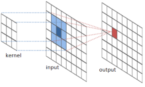
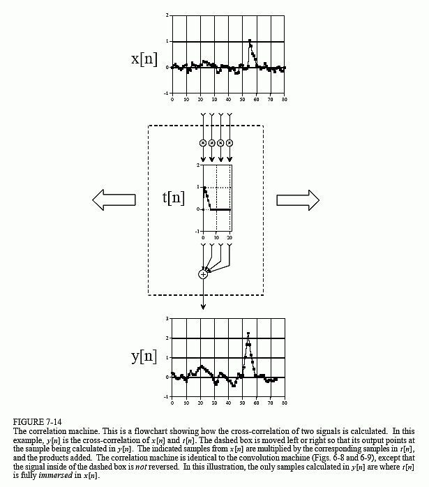
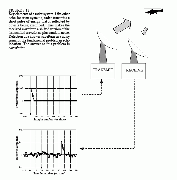
Correlation is a metric for similarity between two different signals, in our case two images.
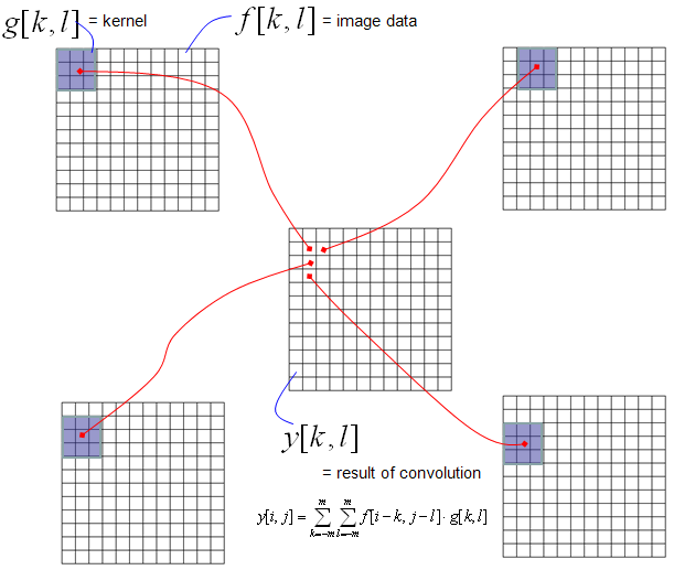
Convolution is correlation with the filter rotated 180 degress.
This makes no difference, if the filter is like a Guassian.
Convolution is associative while correlation is not.
Convolution is multiplication in the frequency domain while, Correlation is the multiplication of the complex conjugate in the frequency domain.

Let's look at some implementation of convolution:

Let's get on to to correlation:
 

 

Project 4.0: Creating tileable draws that match side by side forming a mosaic

In this post, I'll show you another project which you can implement using OpenCV.

There are some intricacies involved, but if you've followed by tutorials till now, it wouldn't be much of a problem.

So, what this project basically involves is creating a Painting tool that allows users to create mosaics.
We need to create tiles of the brush or any pencil tool or any image, side by side.

As I said, if you have followed my tutorials, you can do it yourself.
Please comment below if you have any doubts.

Fourier Theory

The tool, which converts a spatial (real space) description of an
image into one in terms of its frequency components, is called the Fourier transform.
The new version is usually referred to as the Fourier space description of the image.
The corresponding inverse transformation which turns a Fourier space description back into a real space one is called the inverse Fourier transform.
1D Case:
Considering a continuous function f(x) of a single variable x representing distance. The Fourier transform of that function is denoted F(u), where u represents spatial frequency is defined by:

F ( u ) =<integrate from -∞ to ∞> f ( x ) exp(− j 2 π xu) dx

The meaning of this is that, not only is the magnitude of each frequency present important, but that its phase relationship is too.
The inverse Fourier transform for regenerating f(x) from F(u) is given by:

f ( x ) =<integrate from -∞ to ∞> F ( u ) exp(j 2 π xu) du


Some references:
http://homepages.inf.ed.ac.uk/rbf/HIPR2/fourier.htm
https://www.cs.unm.edu/~brayer/vision/fourier.html
http://cns-alumni.bu.edu/~slehar/fourier/fourier.html

Pixels

Neighbors of a Pixel

•  Any pixel p(x, y) has two vertical and two horizontal neighbors, given by (x+1, y), (x-1, y), (x, y+1), (x, y-1)
•  This set of pixels are called the 4-neighbors of P, and is denoted by N 4 (P). Each of them are at a unit distance from P.
•  The four diagonal neighbors of p(x,y) are given by, (x+1, y+1), (x+1, y-1), (x-1, y+1), (x-1 ,y-1).This set is denoted by N D (P).
• The points N D (P) and N 4 (P) are together known as 8-neighbors of the point P, denoted by N 8 (P).
• Some of the points in the N 4 , N D and N 8 may fall outside image when P lies on the border of image.

• (a) 4-adjacency. Two pixels p and q with values from V are 4-adjacent if q is in the set N 4 (p).
• (b) 8-adjacency. Two pixels p and q with values from V are 8-adjacent if q is in the set N 8 (p). 
• (c) m-adjacency (mixed adjacency). Two pixels p and q with values from V are m-adjacent if (i) q is in N 4 (p), or (ii) q is in N D (p) and the set N 4 (p)  ̈ N 4 (q) has no pixels whose values are from V.

Phase II

Hi guys!
Hope you have got your hand on some computer vision techniques.
If you implement it yourself you'll understand better.

I'll begin the next phase of the tutorials.
In this part, I'll cover some more advanced topics which would include some theoretical aspects of computer vision like Transforms, Histogram Equalization, Stereo Vision, Pixel Relations, Pattern Recognition, etc.

So stay tuned!